STPT Data Viewer
The STPT data viewer allows to visualize a dataset obtained with the STPT instrument. Typically these datasets contain large stacks of images of few hundreds of slices in different channels where each image is a mosaic around 20,000 x 20,000 pixels. This 2D viewer offers the possibility to visualize the different slices and select which channels to display in which colour (currently only RGB supported), their intensity scaling as well as the capability to zoom in and visualize the full resolution mosaics.
In order to properly visualize these and allow for user interaction, the STPT pipeline stores multiresolution mosaics that the viewer uses to display the data depending on the level of detail required.
In order to run the viewer in the notebook you need to add the following two lines in a cell at the beginning. The first line loads the module responsible for the viewer and the seconds sets up the environment for output to the notebook.
from imaxt_image.viewer import StptDataViewer, setup_notebook
setup_notebook()
In order to start the viewer we first need to define the dataset name and its location on disk.
dataset_name = "CM1-190610-1302"
directory = "/data/meds1_b/processed/STPT"

dv = StptDataViewer(dataset_name, path=directory)
The main function to display the mosaic is then dv.view. There are a few arguments worth noting:
channels : is a mandatory parameter and it should be a list of three channels that are mapped to the corresponding RGB colour
height : in order to fit the viewer in a Notebook cell we need to set up its height depending on our screen and browser window size. You may need to play with this and with the size of your browser to fit the viewer correctly.
rscale, gscale, bscale : each of these are two element tuples that contain min and max values to display in each channel. If not defined then they are computed automatically.
Typically we would call the function then like:
dv.view(channels=[2,3,4], height=800)
or
dv.view(channels=[2,3,4], rscale=(0.1, 10), gscale=(0.1,30), bscale=(0.1,20), height=800)
and it would produce an output like the one shown below
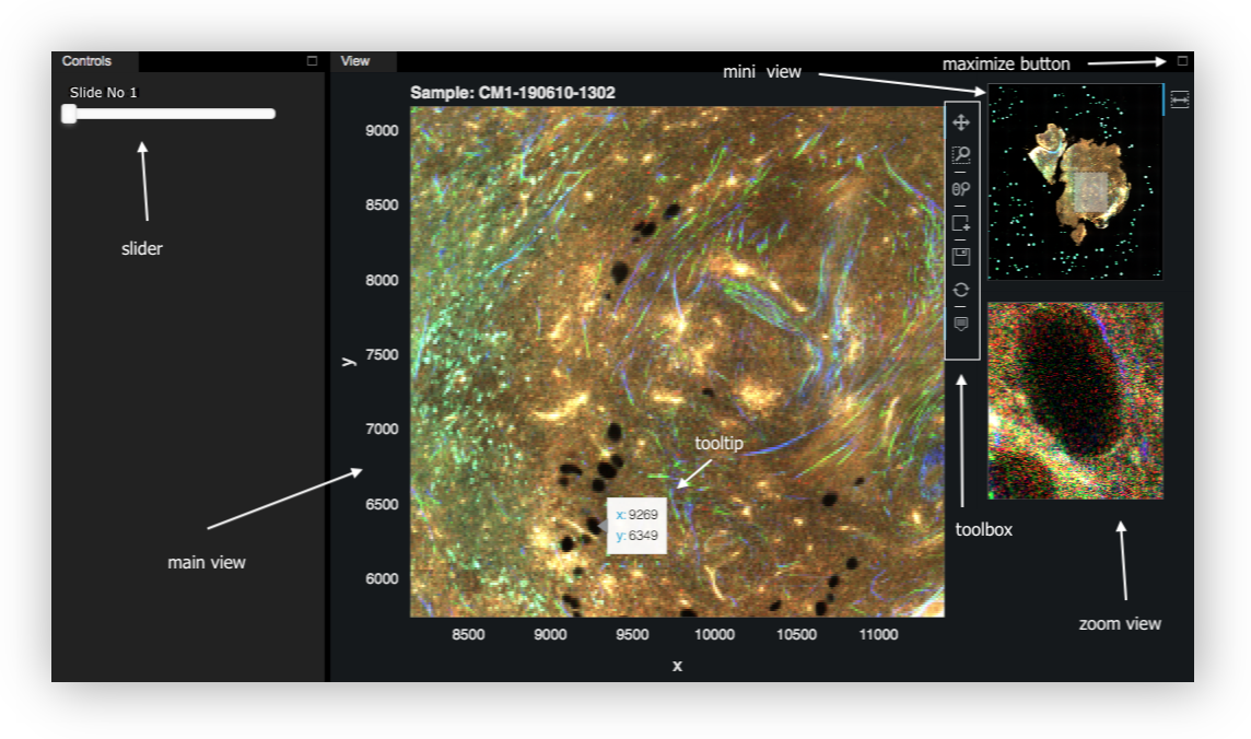
Layout
Slider: The slider on the left allows to navigate through the different slices.
Main view: This contains the RGB made from the selected channels.
Zoom view: displays a full resolution image zoomed on the position of the mouse pointer when it moves over the main view.
Mini view: displays the full range image together with a grey box indicating the area zoomed in. The gray box can be dragged with the cursor to update the main view.
Toolbox: list of tools to interact with the main view
Interactive Controls
The toolbox contains a list of tools that allow a diverse range of interactivity with the main view. Each tool on the toolbox is activated/desactivated clicking on the respective icon with the mouse. You know when a tool is activated because it shows a blue bar at the left of the icon.
 Pan tool: allows the user to pan the plot by left-dragging a mouse across the image region.
 Zoom tool: allows the user to define a rectangular region to zoom the plot bounds to by left-dragging a mouse
 Mouse zoom tool: this tool will zoom the plot in and out, centered on the current mouse location.
 Annotation tool: allows the user to define a rectangular selection region by double clicking and left-dragging a mouse. Once created the box can be moved dragging with the mouse or deleted with Alt + Del.
 Save tool: allows the user to save a PNG image of the plot.
 Reset tool: this will restore the plot ranges to their original values.
 Tooltips tool: this will show a pop up that shows the current (x, y) coordinates of the mouse in the main area
Command line controls
It is possible to use code written in notebook cells to modify and get information from the viewer.
For example, in order to go to slide number 10, run:
dv.goto(10)
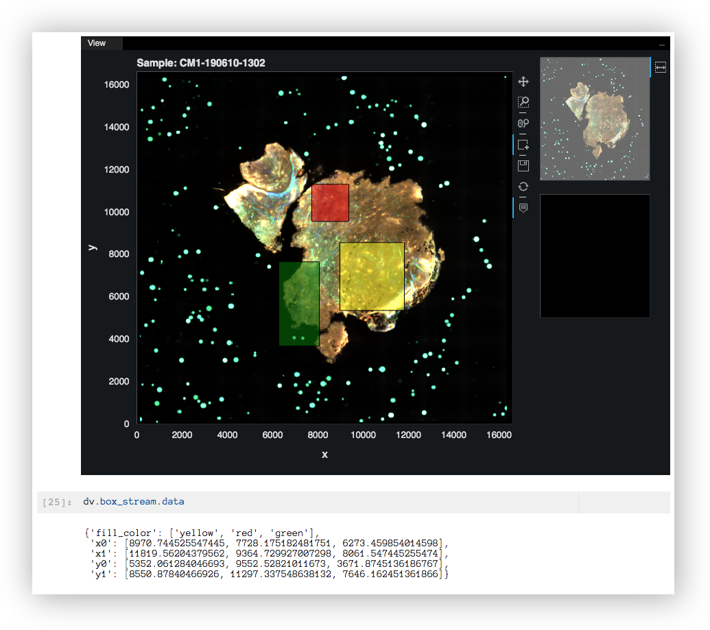
If you draw some boxes on the main window, you can get their coordinates with
dv.box_stream.data
Finally it is also possible to display a series of slices automatically in order and optionally save them as a movie:
dv.play(start=1, end=50, step=1, saveas='test.mp4')
This will display in the viewer the slides (with the current zoom) from number to number 50, one by one, and
saving the result as a movie in MP4 to a file test.mp4. This file is saved as one frame per second.
Follow the link below to open a notebook that goes through an example of visualizing a dataset in JupyterLab.
